By Matt Davis | July 28, 2024
A simpler approach to P50/P99 debt sizing modeling
A core concept for any project finance modeler – and one of the first fundamental skills taught in Pivotal180’s Renewable Energy Project Finance Modeling course – is debt service coverage ratio (DSCR) sculpted debt sizing.
Mathematically, DSCR debt sculpting involves dividing a project’s periodic cash available for debt service (CADS) by a minimum DSCR, and then discounting those future values to the start of the loan repayment period. Because it maximizes leverage for borrowers by creating a debt service profile that effectively matches the shape of project cash flows, DSCR sculpting is utilized for the vast majority of project finance loans.
The minimum DSCR, as well as the interest rate(s) or margin(s) used for discounting future cash flows, are set by the project lender(s). But what about the CADS?
CADS – essentially equal to project revenues less operating expenses, perhaps with a few minor adjustments – are estimated from the project financial model. However, the calculation of CADS is based on a number of uncertain assumptions, most notably energy generation. Future energy generation from any power plant can never be known for certain, and this is especially the case for renewable energy projects where the energy resource – sunshine or wind – varies from month-to-month and year-to-year.
To account for this uncertainty, developers and investors take a statistical approach. Forecasts of annual energy production take the shape of a normal distribution, or bell curve, where the center represents the average annual generation. This value is known as the P50 annual energy estimate, because there is a 50% probability that actual energy will exceed this value on an annual basis. The P50 estimate is often used by equity investors in calculating their base case returns.
Lenders, of course, are concerned with risk, which means they want to consider not just average energy generation, but downside cases. To do this, they typically evaluate CADS under multiple production scenarios: most often, the P50 as well as the P99 estimate, representing the one-in-100 years worst case generation outcome. They then assign separate DSCRs to each CADS estimate and, for debt sizing purposes, take the lesser of CADS divided by DSCR between the two (or more) cases in each period to determine maximum debt service.
Exhibit 1: Maximum debt service based on minimum of CADS/DSCR for P50 and P99 cases
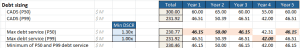
By taking the lesser of multiple DSCR-adjusted CADS cases, lenders protect against downside scenarios that might otherwise result in CADS being insufficient to make debt service payments.
So, how do we deal with this in our models?
The difficult way
Because some revenue and opex items may not scale linearly with energy generation, simply adjusting CADS by a fixed ratio (e.g. 85% if P99 generation is 85% of P50 generation) is often not sufficiently accurate for calculating CADS under multiple scenarios. Many beginning modelers, therefore, spend a great deal of time adjusting their models to enable debt sizing on multiple DSCR criteria. They often replicate all of their operational calculations – generation, revenue, opex, etc. – for each P case and DSCR.
This approach can work, but it is both time consuming and significantly increases the size and complexity of models. Twice as many operational calculations may result in hundreds of additional lines of code within a model. More lines of code also means a greater chance of errors and increases the time needed to review or audit a model and ensure its accuracy.
Fortunately, there is a better approach.
The easy way
Experienced modelers know that a well-designed scenario manager and data table can be used to more efficiently and effectively calculate CADS under multiple production scenarios!
By setting up separate scenarios in our model for both P50 and P99 generation estimates – or any other P cases upon which debt sizing will be evaluated – our model can easily recalculate CADS for each case. Any time we run the P50 case (Case 1, perhaps), live CADS in the model will reflect that generation estimate. If we run the P99 case (Case 2), CADS will automatically be recalculated for the downside case.
Setting up the scenario is the first step, but our work is not done yet. The second step is to create a CADS data table which will calculate CADS for both (or all) of our debt sizing scenarios at the same time. Data tables are often used to compare the results of the model for one or more scenarios or combinations of inputs. While data tables often evaluate just few key model outputs – such as total revenues, debt size, or IRR – we can instead create one to calculate CADS in every period under as many scenarios as we like.
Exhibit 2: CADS data table
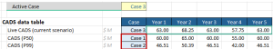
The top row (green border) of our table, “Live CADS,” displays CADS in the currently active case. The lefthand values (red border) are the column inputs for the table – each of the cases we need to calculate the debt size. No matter which case we have active in our model, our CADS data table will always calculate CADS in our debt sizing cases, in addition to the live CADS.
Rather than (perhaps) hundreds of additional rows of operational calculations, a CADS data table does all the work of calculating CADS for the all the cases we need in just a few rows. If our debt sizing criteria change – for example, if a new lender wants to size debt on a P90 case, or a case with higher opex costs – we can easily modify our scenarios and/or our data table to accommodate that.
Additionally, since we can now calculate our debt size from fixed CADS values in our data table, we can run alternative scenarios – such as up/downside operational cases or interest rate sensitivities – without changing our debt size, enabling us to test debt covenants and run sensitivities on returns with a fixed debt quantum and debt repayment schedule. This is critical because debt repayments are fixed in the loan agreement, not variable according to actual project cash flows.
Best of all, setting up this data table takes just a few minutes, rather than hours of time remodeling operations!
Amazing! Tell me more!
Want to learn more about modeling debt sizing for multiple debt covenants, plus more tips and skills to take your debt modeling to another level? Join Pivotal180 for our upcoming Advanced Debt short course, covering this topic plus a range of other debt modeling concepts including:
- leverage limits
- cash sweeps
- leverage sensitivities
- sources and types of debt
- loan agreements and terms
- loan life coverage ratio (LLCR) and debt covenants
- debt service reserve accounts (DSRA).
Want to learn more about project finance, Check out the links below to learn more about Pivotal180 including all of our financial modeling courses and services. Come model with us!